Graphical user interface
Overview
When starting the program, the user is presented with the following interface (minus the markings).
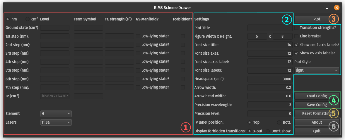
The window is divided into several components:
- The main area to define the laser ionization scheme.
- Settings and configurations for how to display the plot. These are pre-filled with some reasonable defaults.
- The button to plot and show the figure.
- Buttons to load and save configurations.
- A button to set the formatting settings back to the default values.
- Buttons to get information about the program and to quit the program.
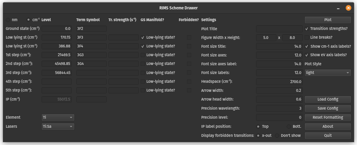
An example of the filled in GUI can be seen here and is discussed further below.
Resonance ionization scheme
The scheme can be set up in the left hand side of the program. The following shows a marked up version of this part:
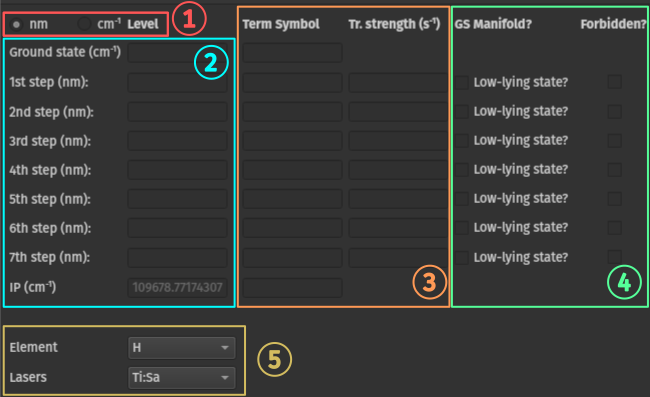
The sections are as follows:
- Unit selection: Please select if you want to enter the transitions in nm or in cm-1.
- Here you can enter the states / transitions. The units that need to be entered are automatically updated if you change the selection in 1.
- In the left column, please give the term symbol of the state that should be displayed. On the right, please enter the transition strength in s-1. Note that To display the transition strength in the plot, the according box in the settings (see below) must be checked.
- If the ground state manifold contains low-lying states, please check the left box in this section. The state must then be given in cm-1. If a transition is forbidden, you can additionally check the "Forbidden?" box.
- As you can see for the IP level in 1, the ionization potential is automatically set. We currently include all elements with IPs define in the NIST Atomic Spectra Database. Finally, please select the lasers that were used for this scheme. While this is unimportant for the plot, it is used when submitting a scheme to the online database.
Settings of the plot
The settings of the plot can be configured on the right-hand side of the program, labeled 2 in the overview image. The following settings from top to bottom in the left column are available.
- Plot title: Here you can enter an optional title for the plot.
- Width and height of the figure. This is set in inches, however, the actual units are fairly unimportant.
- Font size of the title (if set).
- Font size of the axes.
- Font size of the axes labels.
- Headspace in cm-1. This is the space above the IP that will be added. This is one of the most frequent values changed in the settings. For example, you might want to add additional space in order to display all labels nicely within the plot.
- Width of the arrow in arbitrary units. Mainly needs to be changed if the figure size is modified.
- Arrow head width in arbitrary units. Mainly needs to be changed if the figure size is modified.
- Precision of the wavelength: How many digits should be displayed for the wavelengths?
- Precision of the levels: How many digits should be displayed for the levels?
- Where should the IP be labeled: on top or on the bottom of the IP line?
- How do you want to show forbidden transitions? Cross them out ("x-out") or don't show them at all ("Don't show")?
In the right column, the following options are available:
- Transition strengths? Checkbox to display the transition strengths in the plot.
- Line breaks? Checkbox to show line breaks between the levels and the term symbols. This can be useful if you want a narrow figure or higher level precision.
- Show cm-1 axis labels? If unchecked, the left axis labels will disappear.
- Show eV axis labels? If unchecked, the right axis labels will disappear.
- Plot style: Please select from the dropdown menu, how you want to style your plot. The default is "light". If you select a transparent option, the plot background will be transparent (useful for talks with non-black/non-white backgrounds).
Note
The filled GUI example image above shows a reasonable setup for a Ti resonance ionization scheme (plot shown below). Note especially the setup for the low-lying states and the term symbols that were entered.
Show axis labels
The "Show axis labels" as described above can be useful in case you need to combine multiple schemes into one figure.
In this case, create multiple figures with the same figure height.
Then, calculate the headspace for each figure, such that the cm-1 of the maximum height align in each figure.
The total height of the figure will always be IP level + headspace.
Finally, save the figure (see below), e.g., as an svg file and combine the figures with a vector graphics editor.
Plotting
Once the scheme is filled out, hit the "Plot" button in order to display a figure. A window will open with the figure. Here's an example:
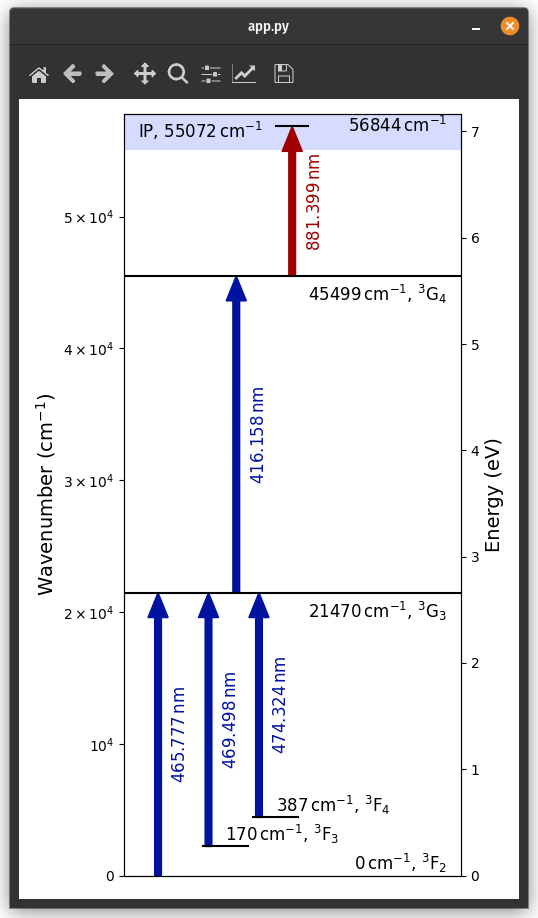
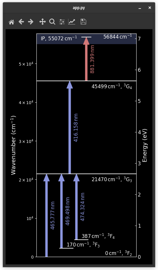
This figure is for a Ti resonance ionization scheme, taken from Trappitsch et al. (2018). The setup of the GUI to create this scheme can be found above.
To save this figure, you can use the floppy disk
icon in the toolbar of the figure window.
The available formats can be found here.
Recommended saving formats are png for pixel graphics and svg or pdf for vector graphics.
Saving and loading configurations
If you want to save a given configuration, you can use the "Save Config" button.
The data will be saved as a json file.
You can open a saved file with any text editor and have a look,
but please note that bad things can happen if you change the file right there,
unless of course you know what you're doing.
The file should be fairly self-explanatory.
To load a given configuration, you can use the "Load Config" button. This will open a file dialog where you can select the file to load.
The configuration file for the example titanium scheme shown above can be found here.